Unit 2: Supply and Demand

Created	@September 20, 2021 9:46 AM
Tags	In Class

2.1 - Key Terms

Quantity Demanded

Quantity demanded is the amount of a good demanded by buyers at a given price level.

Buyers who are:

Willing to buy

Able to buy

Combine to make the Effective Demand.

Quantity demanded is the effective demand at a given price level. Quantity demanded has an inverse relationship with price.

💡

Price moves Quantity Demanded. Price is the independent variable in this equation, and Quantity Demanded is the dependent one. Consumers are reactive to changes in price.

Paradox of Demand

Under the paradox of demand, some goods do not have an inverse relationship between price and quantity demanded, but a parallel relationship. Goods are bought at higher prices in order to impress others, for things like luxury goods, therefore demand increases as price increases.

There are two causes for the paradox of demand, either conspicious consumption (buying goods to impress others), or Giffin goods (inferior goods which have no close substitutes).

Demand Schedule

A table showing how much of a good or service consumers will want to buy at different prices.

Graphing Price vs. Quantity Demanded

Price goes on the y-axis, quantity demanded goes on the x-axis.

This is known as a demand curve.

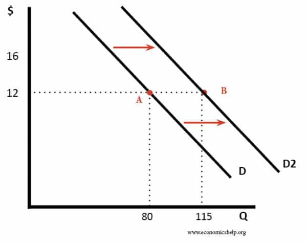
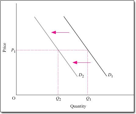
When there is an increase in demand, the demand curve shifts right (outward), with $D_0$ being the original curve and $D_1$ being the new curve. The opposite is also true, when there is a decrease in demand, the demand curve shifts left (inward).

Therefore, when total demand increases, the quantity demanded will increase at ALL POSSIBLE price levels. This means that something other than price has caused consumer demand to increase. The same is, of course, possible for a decrease in demand.

Causes of Change in Demand

Something other than price changes:

I: Income - Consumer Income Changes
- With an increase in Consumer Income: Curve shifts right for Normal Goods (Fettuccini Alfredo) & Left for Inferior Goods (Ramen)
- With a decrease in Consumer Income: Curve shifts left for Normal Goods & right for Inferior Goods

N: Number - Change in the Number of Consumers
- Increase in number of buyers: Curve shifts right
- Decrease in number of buyers: Curve shifts left

S: Substitute - Change in the Price of Substitute Goods
- Increase in the price of substitutes: Curve shifts right
- Decrease in the price of substitutes: Curve shifts left

E: Expectations - Change in expectations of future price
- Expect a rise in price: Curve shifts right
  - Gonna buy up before price goes up
- Expect a decrease in price: Curve shifts left
  - Not gonna buy until price decreases

C: Complement - Change in the price of complement goods
- Two goods that go together will move in opposite directions as the price of the other changes.

T: Taste - Change in consumer taste and preferences
- Increase in Taste or Preference for the item: Curve moves Right
- Decrease in Taste or Preference for the item: Curve moves Left

Income Effect

The income effect is the change in the consumption of goods by consumers based on their income. When the price of a good falls, consumers experience an increase in purchasing power from a given income level. When the price of a good increases, consumers experience a decrease in purchasing power.

Normal goods have a positive income effect, that is, more of the good is consumed as the income of it's consumers increases. Inferior goods have a negative income effect, as consumers' income increases, less of the good is purchased.

Substitution Effect

The substitution effect happens when consumers replace cheaper items with more expensive ones when their financial conditions change. When the price of a good falls, consumers will substitute toward that good and away from other goods.

2.2 - Supply

Law of Supply

The quantity supplied of any good is the amount that sellers are willing and able to sell.

The Law of Supply states that the quantity supplied of a good rises when the price of the good rises, other things being equal.

The Supply Schedule

A supply schedule is a table that shows the relationship between the price of a good and the quantity supplied. These tables have two columns, the price of the good and the quantity supplied.

Market Supply vs. Individual Supply

The quantity supplied in the market is the sum of the quantities supplied by all the sellers at each price.

$Q^s$ represents the market quantity supplied

Supply Curve Shifters

The supply curve shows how price affects quantity supplied, other things being equal.

These other things are the non-price determinants of quantity supplied. \

Input Prices

Examples of input prices: wages, prices of raw materials

A fall in input prices makes production more profitable at each output price, so firms supply a larger quantity at each price, and the $S$ curve shifts to the right.

An increase in input prices makes production less profitable at each output price, so firms supply a lower quantity at each price, and the $S$ curve shifts to the left.

Technology

Technology determines how much inputs are required to produce a unit of output.

A cost-saving technological improvement has the same effect as a fall in input prices, it shifts the $S$ curve to the right.

Number of Sellers

An increase in the number of sellers increases the quantity supplied at each price.

This also shifts the $S$ curve to the right.

Expectations

An expectation of a higher price for a good will cause sellers to reduce their quantity supplied and hold on to their inventory until the price increases, temporarily shifting the $S$ curve to the left.

This only applies if the goods are not perishable

Summary: Variables that Influence Sellers

Change in price causes a movement along the $S$ curve

Fancy Acronym

R - Resource Input/Cost

O - Other goods

T - Technology

T - Taxes

2.3 - Price Elasticity of Demand

Elasticity measures how much one variable responds to changes in another variable.

In economics, elasticity is a numerical measure of the responsiveness or $Q_d$ or $Q_S$ to one of its determinants.

Price elasticity of demand measures how much $Q_d$ responds to a change in $P$ .

\textrm{Price elasticity of demand} = \frac{\textrm{Precentage change in } Q_d}{\textrm{Percentage change in } P}

Loosely speaking, it measures the price sensitivity to buyer's demand.

Along a $D$ curve, $P$ and $Q$ move in opposite directions, which would make price elasticity negative.

We will drop the minus sign and write all demand elasticities as positive numbers.

Calculating Percentage Changes

Standard method of computing the percentage change:

\frac{\textrm{end value} - \textrm{start value}}{\textrm{start value}} \times 100\%

🙄

AP Graders are really picky and want to see all of your work so make sure you actually show the formulas and the work with numbers plugged in.

This method sucks though so we will use the midpoint method for elasticity instead.

\frac{\textrm{end value} - \textrm{start value}}{\textrm{midpoint}} \times 100\%

Where the midpoint is the number halfway between the start and end values, the average of those values.

\frac{\textrm{end value} - \textrm{start value}}{(\textrm{end value} + \textrm{start value})/2} \times 100\%

Determinants of Price Elasticity

The extent to which close substitutes are available

Whether the good is a necessity or a luxury

How broadly or narrowly the good is defined

The time horizon -

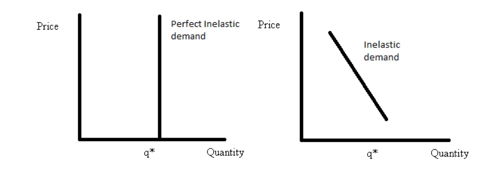
Inelastic Demand

When the price elasticity of demand is <1, it is considered inelastic demand. That is, the customer's sensitivity to price is relatively low.

When $D$ is inelastic, a price increase causes revenue to grow.

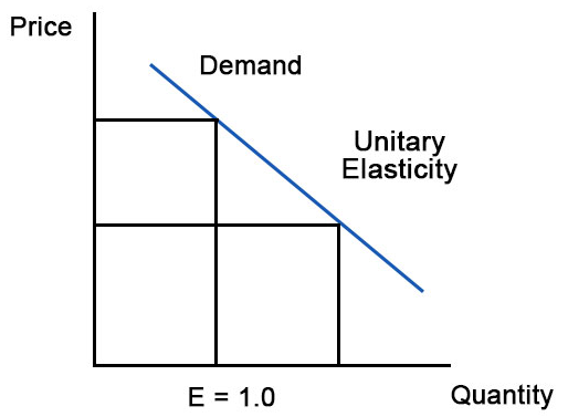
Unit Elastic Demand

When the price elasticity of demand =1, this is considered unit elastic demand. This means that consumer's sensitivity to price is intermediate. A change in price with unit elastic demand has no effect on revenue for businesses.

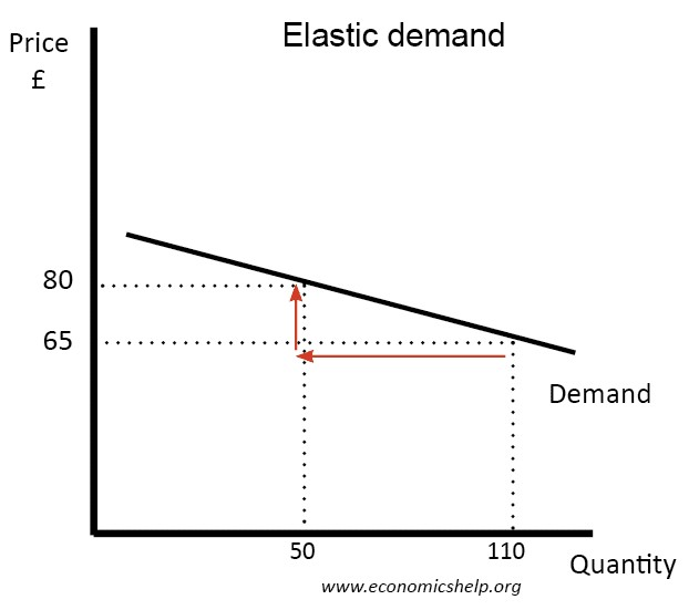
Elastic Demand

When the price elasticity of demand >1, this is considered elastic demand. Price sensitivity is relatively high. The change in $Q_D$ is greater than the change in $P$ .

When $D$ is elastic, a price increase causes revenue to fall.

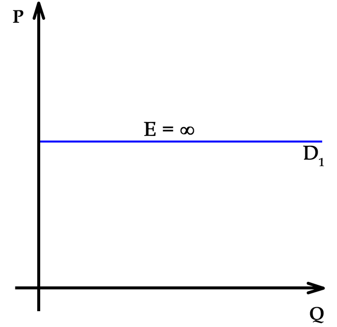
Perfectly Elastic Demand

When the $D$ curve is completely horizontal, the price elasticity of demand = $\infin$ and consumer's price sensitivity is extreme.

2.4 - Price Elasticity of Supply

Perfectly Inelastic Supply

\textrm{Price elasticity of supply} = \frac{\textrm{\% change in Q}}{\textrm{\% change in P}} = \frac{0\%}{10\%} = 0

$S$ curve is vertical

Seller's price sensitivity is zero

Inelastic Supply

\textrm{Price elasticity of supply} = \frac{\textrm{\% change in Q}}{\textrm{\% change in P}} = \frac{<10\%}{10\%} < 1

$S$ curve is relatively steep

Seller's price sensitivity is relatively low

Unit Elastic Supply

\textrm{Price elasticity of supply} = \frac{\textrm{\% change in Q}}{\textrm{\% change in P}} = \frac{10\%}{10\%} = 1

$S$ curve has an intermediate slope

Seller's price sensitivity is intermediate

Elastic Supply

\textrm{Price elasticity of supply} = \frac{\textrm{\% change in Q}}{\textrm{\% change in P}} = \frac{>10\%}{10\%} > 1

$S$ curve has a relatively flat slope

Seller's price sensitivity is relatively high

Perfectly Elastic Supply

\textrm{Price elasticity of supply} = \frac{\textrm{\% change in Q}}{\textrm{\% change in P}} = \frac{\textrm{any} \space \%}{0\%} = \infin

$S$ curve is horizontal

Seller's price sensitivity is infinite

Determinants of Supply Elasticity

The more easily sellers can change the quantity they produce, the greater the price elasticity of supply.
- Example: Supply of beachfront property is harder to vary and thus less elastic than supply of new cars.

For many goods, price elasticity of supply is greater in the long run than in the short run, because firms can build new factories, or new firms may be able to enter the market.

2.5 - Other Elasticities

Income Elasticity of Demand

Measures the response of $Q_d$ to a change in consumer income.

\textrm{Income elasticity of demand} = \frac{\textrm{Percent change in } Q_d}{\textrm{Percent change in income}}

For normal goods, the income elasticity of demand is > 0 (positive), while for inferior goods, the income elasticity of demand is < 0 (negative).

Cross-price Elasticity of Demand

Measures the response of demand for one good to changes in the price of another good.

\textrm{Cross-price elasticity of demand} = \frac{\textrm{Percent change in } Q_d \textrm{ for good 1}}{\textrm{Percent change in price for good 2}}

For substitutes, cross-price elasticity > 0 (e.g. an increase in price of beef causes an increase in demand for chicken)

For complements, cross-price elasticity < 0 (e.g. an increase in the price of computers causes a decrease in demand for software)

2.6 - Market Equilibrium and Consumer and Producer Surplus

Surplus (excess supply)

When quantity supplied is greater than quantity demanded, surplus is the excess quantity supplied that is not demanded. Any price above equilibrium creates a surplus. Price will eventually decrease until it stabilizes at equilibrium.

Shortage (excess demand)

When quantity demanded is greater than quantity supplied, the difference between quantity demanded and quantity supplied is the shortage. Any price below equilibrium will create a shortage. Price will eventually increase to reach equilibrium again.

Willingness to Purchase (WTP)

Willingness to purchase is the measure of the highest price at which a buyer is willing to purchase a good. At any $Q$ , the height of the $D$ curve is the WTP of the marginal buyer.

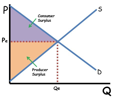
Consumer Surplus (CS)

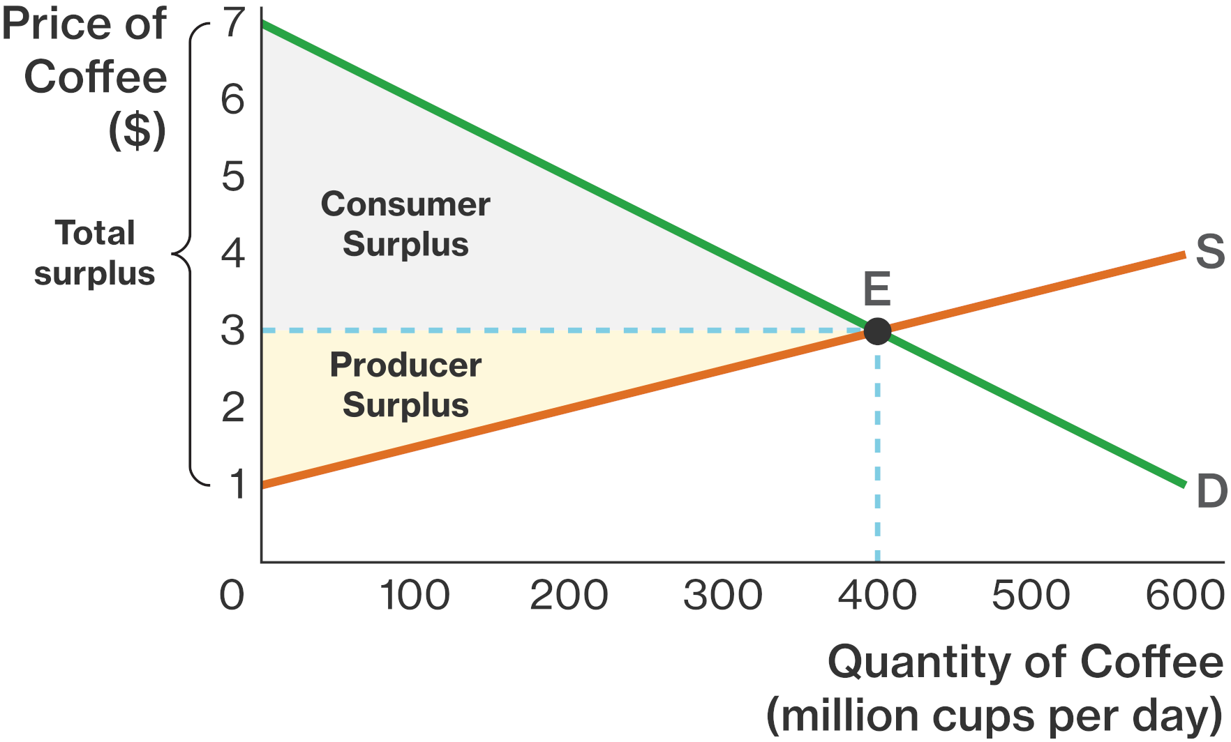
Consumer surplus is the amount a buyer is willing to pay minus the amount the buyer actually pays.

CS = WTP - P

On a demand curve, the consumer surplus is the area above the given price but below the demand curve, from $0$ to $Q$ .

Cost and the Supply Curve

Cost is the value of everything a seller must give up to produce a good (i.e. opportunity cost). This includes the cost of all resources used to produce the goods, including the value of the seller's time.

A seller will produce and sell the good/service only if the price exceeds the cost, that is, they can make a profit.

At each $Q$ , the height of the $S$ curve is the cost of the marginal seller, the seller who would leave the market if the price were any lower.

Producer Surplus

Producer surplus equals the price of a good minus the cost of it's production.

PS = P - C

On a supply curve, the producer surplus is the area above the supply curve and below the price of the good.

2.7 - Market Disequilibrium and Changes in Equilibrium

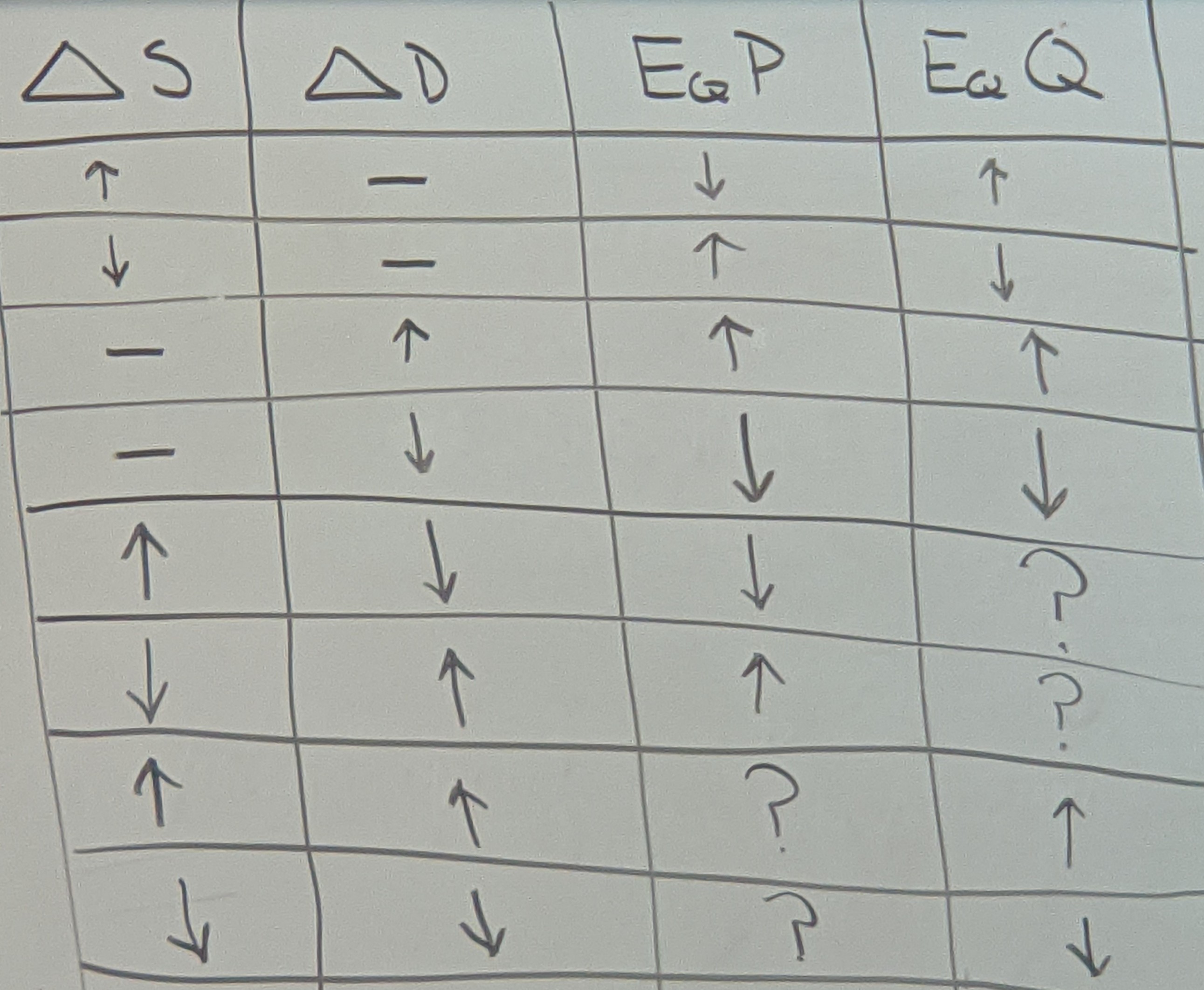
Effects of a change in Supply or Demand

Total Surplus & Efficiency

The total surplus is the sum of consumer and producer surplus.

\textrm{TS} = \textrm{CS} + \textrm{PS}

Another way of putting this is that the total surplus is the value to buyers minus the cost to sellers.

\textrm{Total surplus} = (\textrm{value to buyers}) - (\textrm{cost to sellers})

An allocation of resources is efficient if it maximizes the total surplus. Efficiency means:

The goods are consumed by the buyers who value them most highly.

The goods are produced by the producers with the lowest costs.

Raising or lowering the quantity of a good would not increase the total surplus.

2.8 - The Effects of Government Intervention in Markets

When the equilibrium price of a good is deemed too high by a government, they will put in place a price ceiling below the natural equilibrium price (binding). This is a maximum price of a good in a market. Instituting a price ceiling will create a shortage, as now $Q_S$ is less than $Q_D$ .

Effects of a Tax

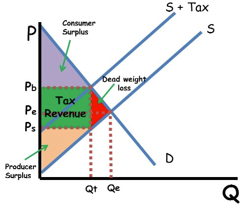
The size of a tax can be represented by $\$T$ . The government's revenue from tax is represented by:

\$ T \cdot P_T

With a tax, both $CS$ and $PS$ are reduced, and the area between them is the tax revenue. The area to the right of the tax revenue becomes dead weight loss.

Taxes can be considered a form of surplus, and therefore are incorporated into total surplus.

Deadweight Loss

The goods between $Q_E$ and $Q_T$ are not sold, and are known as the deadweight loss.

The size of the deadweight loss is determined by the price elasticities of supply and demand.

When supply is inelastic, it is harder for firms to leave the market when the tax reduces $P_S$ , and therefore the DWL is low. The more elastic the supply, the easier it is for firms to leave the market, and thus there is a higher change in $Q$ and a higher DWL.

When the demand is inelastic, it's harder for consumers to leave the market when the tax raises $P_B$ . So, the tax only reduces $Q$ a little, and the DWL is small. The more elastic the demand, the easier for buyers to leave the market, and thus there is a higher change in $Q$ and a higher DWL.

Depicted on a Graph

2.9 - International Trade and Public Policy

$P_W$ = the world price of a good, the price that prevails in world markets.

$P_D$ = domestic price without trade.

If $P_D \lt P_W$
- country has a comparative advantage in the good
- under free trade, country exports the good

If $P_D \gt P_W$
- country does not have a comparative advantage in the good
- under free trade, the country will import the good

The Small Economy Assumption

A small economy is a price taker in world markets: Its actions have no effect on $P_W$ .

Not always true, but simplifies the analysis

The Welfare Effects of Trade

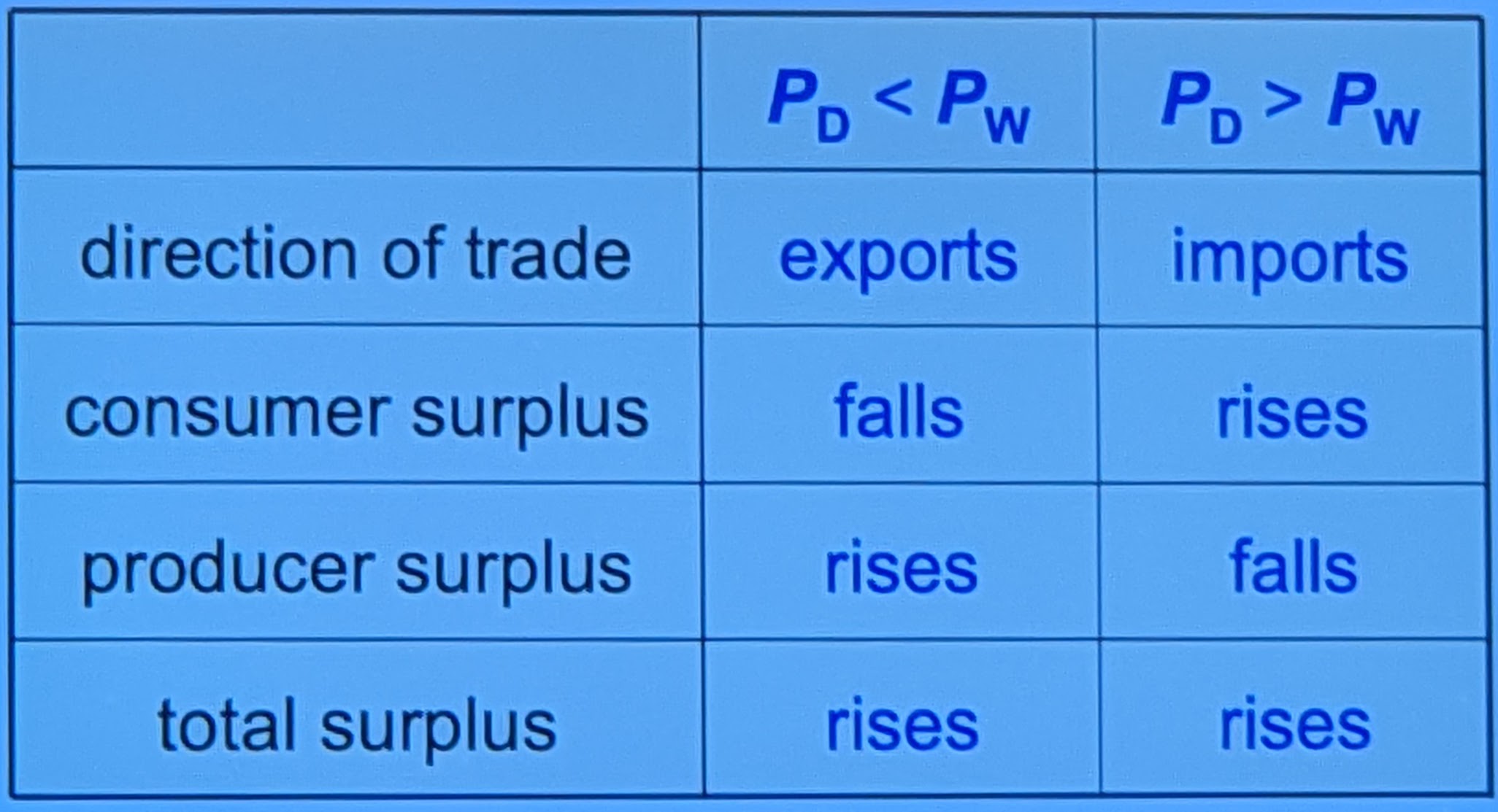
When a good is imported or exported, trade creates winners and losers.

Other Benefits of International Trade

Consumers enjoy an increased variety of goods

Producers sell to a larger market and may achieve lower costs

International competition may increase market power of local producers

Tariff: An Example of a Trade Restriction

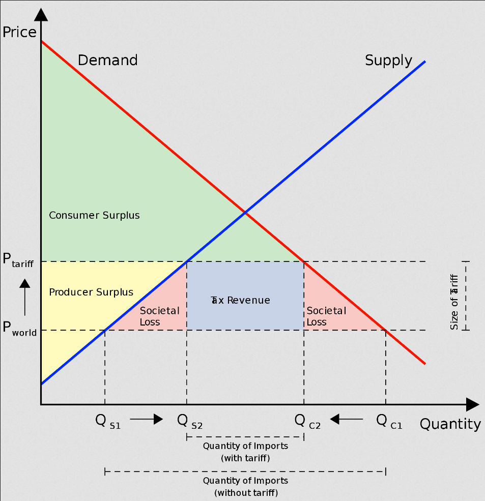
A tariff is a tax on imports.

Example: Cotton shirts
- $P_W = \$20$
- Tariff: $T = \$10/\textrm{shirt}$
- Consumers must pay $30 for an imported shirt.
- Therefore, domestic producers can charge $30 per shirt.

In general, the price facing domestic buyers & sellers equals $P_W + T$ .

Effect of a Tariff on Supply and Demand

Arguments for Restricting Trade

Trade destroys jobs in industries that compete with imports.
- Look at the data. Do rising imports cause rising unemployment? No.
- Imports do not destroy jobs, only change which jobs are available.

An industry vital to national security should be protected from foreign competition, to prevent dependence on imports.
- Producers may exaggerate their own importance to national security to get protections

A new industry argues for temporary protection until it's mature and can compete with foreign firms
- This is dumb — Sincerely, Economists

Producers argue their competitors in another country have an unfair advantage
- Ok perfect that sucks we're just gonna import and you suck go die — Economists

Nation could use restricting trade to bargain with other nations
- This is a bad idea, as it places the nation between a rock and a hard place if the other nation declines to act.

Trade Agreements

A country can liberalize trade with
- unilateral reductions in trade restrictions
- multilateral agreements with other nations

Examples of trade agreements:
- North American Free Trade Agreement (NAFTA), 1993
- General Agreement on Tariffs and Trade (GATT), ongoing