3.0 - Overview & Market Structures

Perfect Competition

• Many firms in competition with each other

• Goods being sold are identical, with no product differentiation

• Individual firms have no control over prices, they are called "price takers"

• Low barrier to entry (solely startup cost)

• Well informed buyers and sellers

Monopolistic Competition

• Many firms in competition with each other

• There is some amount of differentiation between products

• Individual firms have no control over prices, they are called "price takers"

• Low barrier to entry (solely startup cost)

• Monopolistic competitors use non-price competition (Advertising, giveaways, promotions, etc.)

Oligopoly

• Few firms control the market

• Firms have a strong control over price, and frequently collude to set prices

• Firms can also engage in price wars and predatory pricing

• Medium barrier to entry

• Price Leadership: Unofficial collusion where firms follow a single firm when that firm changes their price

Monopoly

• One firm has absolute control over the market

• No variety of goods

• Firm is a price maker, they are able to set the price to whatever they want

• High barrier to entry

3.1 - The Production Function

Vocabulary

• Inputs—Any resources (and, labor, capital, or entrepreneurship) that is used by firms to produce outputs. Ex: a pizza parlor needs inputs such as tomatoes, yeast, and flour.

• Costs—Money that is spent to purchase inputs. Ex: in order to get workers (labor) you have to pay wages (a type of cost).

• Outputs—The finished goods and services that firms produce in order to make revenue. Ex: a toy company's outputs are different types of toys.

• Revenue—This the all money received by a firm (Price x Quantity). Ex: If Mattel sells their Barbie doll for $10 and they sell 100 of the dolls, then their revenue is $1000.

Total, Average, and Marginal Product

Total product (TP)—the total quantity of output produced by a firm in the market.

Average product (AP)—The quantity of total output produced per unit of input used in the production process (Total Product / Units of Inputs).

Marginal product (MP)—The quantity of total output produced by each additional unit of input used in the production process. This is calculated by dividing the change in total product by the change in quantity of input.

The Production Function

The Theory of Production is the idea that input is related to output.

A Production Function shows the relationship between the quantity of inputs used to produce a good and the quantity of output of that good.

The slope of the production function represents the marginal product of labor, the change in output that results from employing an added unit of labor.

In continuous terms, the $\textrm {MP}_L$ is the first derivative of the production function 🤯.

$\textrm{MP}_L$ diminishes as $L$ increases due to the law of diminishing marginal returns.

Law of Diminishing Marginal Returns

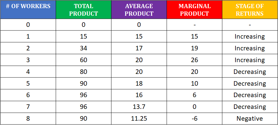
Increasing Marginal Returns—Each additional variable input is more productive than the last. MP and AP increase, as each variable input specializes in its task and utilizes fixed inputs. TP increases at an increasing rate.

Decreasing Marginal Returns—Each additional variable input is less productive than the last. MP and AP decrease as specialization decreases, and there are not enough fixed inputs. TP increases, but at a slower rate.

Negative Marginal Returns—Each additional variable input gets in the way of production. AP decreases and MP becomes negative, as specialization is impossible with too many variable inputs. TP decreases.

The Law of Diminishing Marginal Returns dictates that, as variable resources are added to fixed resources, the additional output produced from each new input will eventually fall. Basically, at some point, each additional worker used in the production process becomes less productive.

Stages of Marginal Returns

• Stage 1: Increasing Marginal Returns. Both TP and MP are increasing.

• Stage 2: Diminishing Marginal Returns. TP is still increasing, but MP is decreasing.

• Stage 3: Negative Marginal Returns. Both TP and MP are decreasing.

Graphs of the Production Function

Relating Total, Average, and Marginal Products

Relationship between Marginal Product and Total Product

The law of variable proportions explains the relationship between Total Product and Marginal Product. It states that when only one variable factor input is allowed to increase and all other inputs are kept constant, the following can be observed:

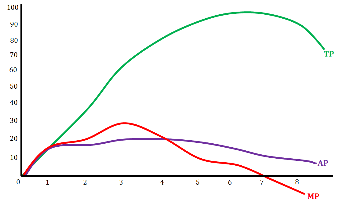
• When the Marginal Product (MP) increases, the Total Product is also increasing at an increasing rate. This gives the Total product curve a convex shape in the beginning as variable factor inputs increase. This continues to the point where the MP curve reaches its maximum.

• When the MP declines but remains positive, the Total Product is increasing but at a decreasing rate. This gives the Total product curve a concave shape after the point of inflection. This continues until the Total product curve reaches its maximum.

• When the MP is declining and negative, the Total Product declines.

• When the MP becomes zero, Total Product reaches its maximum.

Relationship between Average Product and Marginal Product

There exists an interesting relationship between Average Product and Marginal Product:

• When Average Product is rising, Marginal Product lies above Average Product.

• When Average Product is declining, Marginal Product lies below Average Product.

• At the maximum of Average Product, Marginal and Average Product equal each other.

3.2 - Short-Run Production Costs

In the short-run, at least 1 resource is fixed, or cannot change. Fixed resources can include plant capacity, or the number of factories in operation.

Fixed, Variable, and Total Costs

Fixed Cost (FC)—The costs of fixed resources used during the production process. These costs do not change with the amount of output produced. Ex: rent, salaries, insurance.

Variable Cost (VC)—The costs of variable resources used during the production process. These costs do change with the amount of output produced. The more output produced, the higher the variable costs are and vice versa. Ex: electricity, hourly wages, shipping costs.

Total Cost (TC)—The sum of variable costs and fixed costs.

Marginal Cost (MC)—The additional cost of producing each additional unit of output. ($\textrm{MC} = \frac{\Delta TC}{\Delta Q}$)

Relating Fixed, Variable, and Total Costs

Average Costs

Average Fixed Cost (AFC)—Fixed cost divided by the quantity of output

Average Variable Cost (AVC)—Variable cost divided by the quantity of output.

Average Total Cost (ATC)—Total cost divided by the quantity of output.

Economic Profit vs. Accounting Profit

Implicit cost—Opportunity costs associated with decisions in the production of goods and services. Ex: If an individual gives up an annual salary to open a business, then that salary is seen as an implicit cost.

Accounting costs—The explicit or "out of pocket" payments paid by firms to use resources during the production process.

Economic costs—The sum of both the implicit costs (opportunity costs) and explicit costs of production. These costs include both the "out of pocket" payments paid by firms and the opportunity costs of using resources during the production process.

Accounting profits—The profits earned by the firm when the revenue earned by the firm is greater than the explicit (accounting) costs of production (Total Revenue - Accounting Costs).

Economic profits—The profits earned by the firm when the revenue earned by the firm is greater than the sum of the explicit (accounting) costs and the implicit (opportunity cost) costs of production (Total Revenue - Economic Costs).

Accounting profits ignore the implicit costs, and therefore will always appear higher than economic profit.

Graphical Depictions of Fixed, Variable, and Total Cost

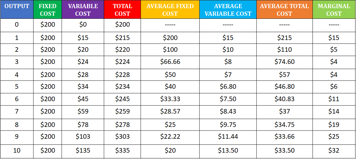
Example table of a firm's FC, VC, and TC, and how those are related to the firm's output.

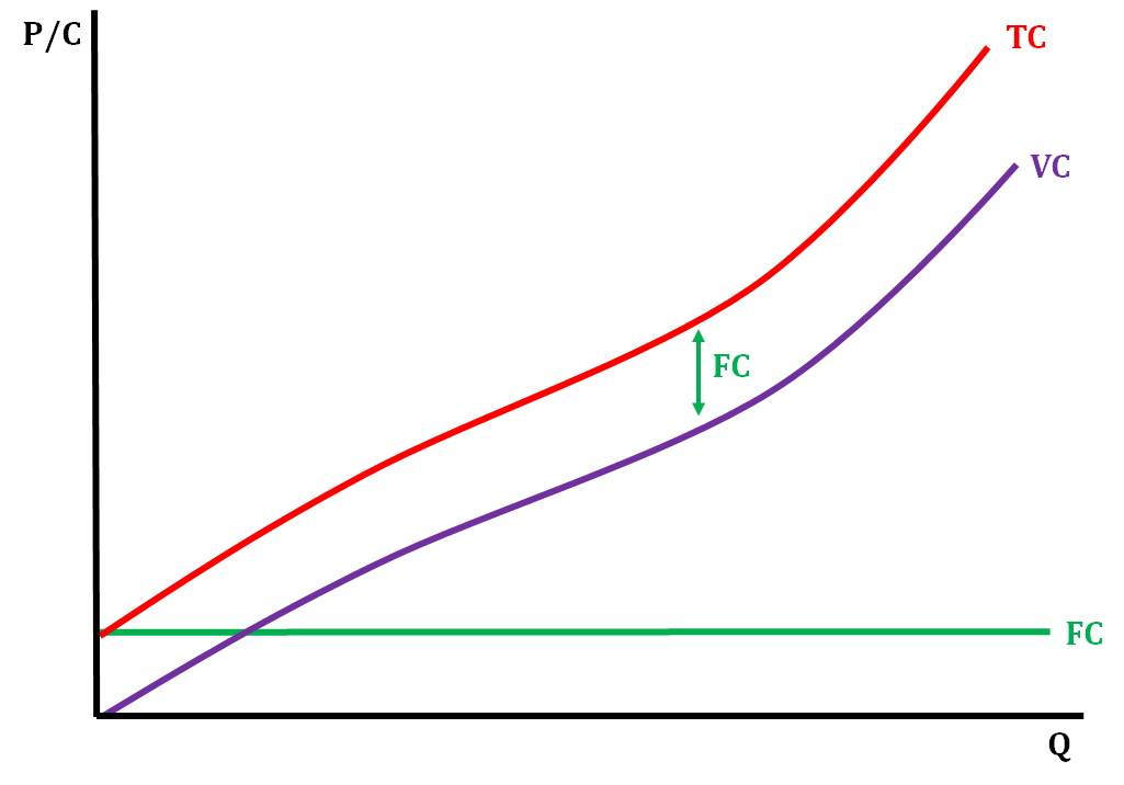
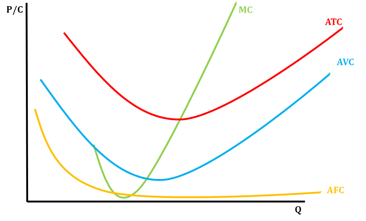
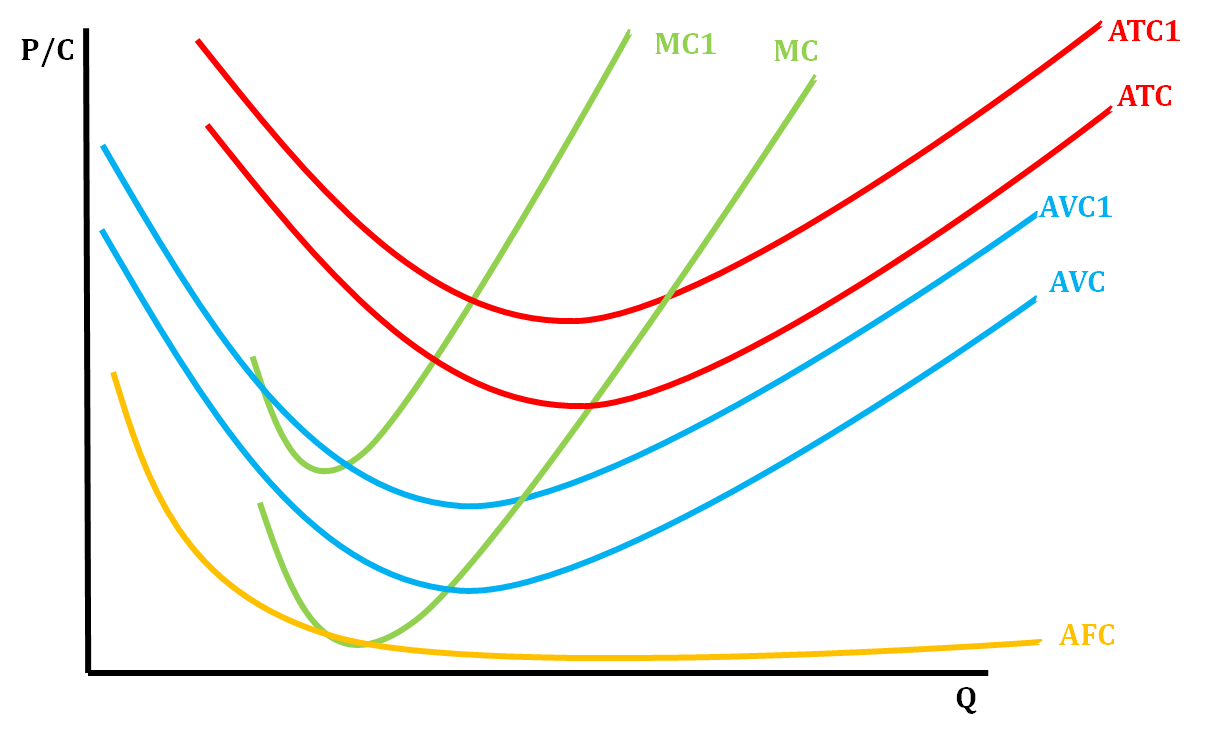
MC always crosses both AVC and ATC at their lowest point. If fixed costs increase, then both the AFC and ATC would shift up and vice versa. If variable costs increase, then both AVC and ATC will shift upward and vice versa. The MC curve only shifts when variable costs change. It will shift upward for an increase in variable costs and downward for a decrease in variable costs.

3.3 - Long-Run Production Costs

In the long-run, all resources are flexible, so firms can change both their plant capacity and output level. This allows firms to analyze and compare the average total cost of production at each plant capacity in the short-run, and find the optimal plant capacity that allows them to product output at the lowest possible ATC.

This the LRATC curve is merely the combination of several SRATC curves for different facilities.

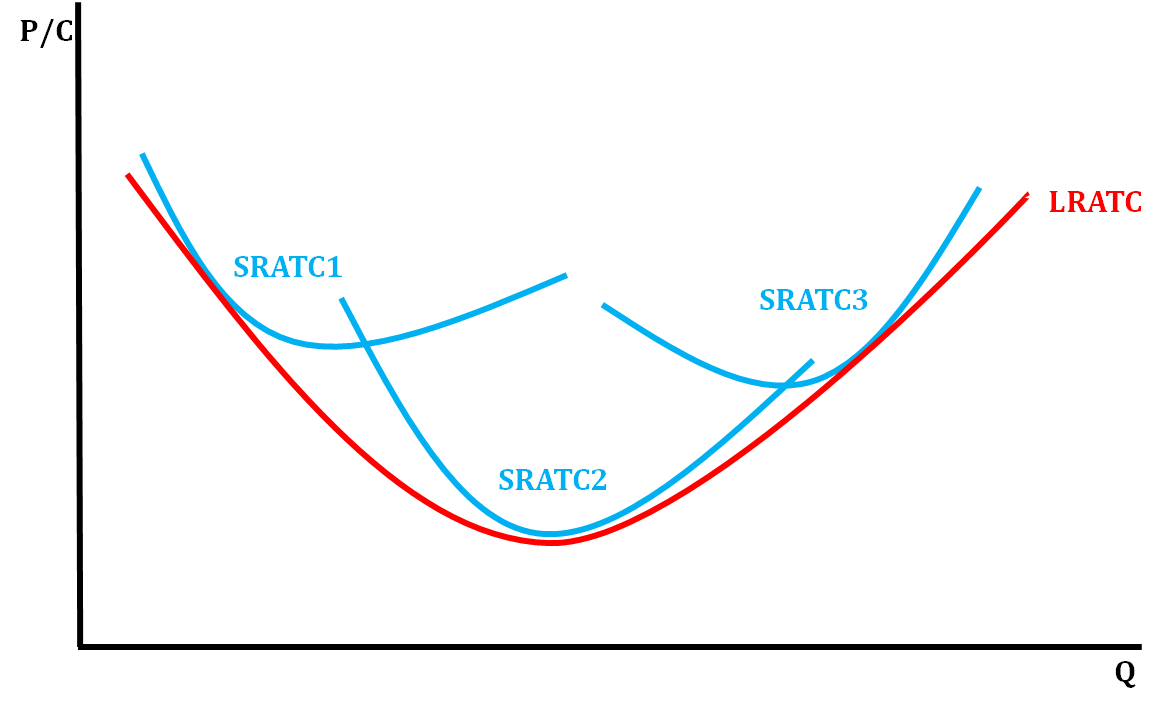
The U-shape of the long-run ATC (LRATC) curve is a result of economies of scale and diseconomies of scale that are experienced by the firm.

• Economies of scale refers to the reduction in total cost-per-unit as a firm increases its production. In this phase, the firm can reduce its total cost-per-unit by boosting its plant capacity and output.

• Diseconomies of scale refers to the rise in total cost-per-unit as the firm increases its production. In this phase, the firm would be better off reducing its plant capacity and output in order to lower their per-unit costs.

• In between these two phases is what we refer to as constant returns to scale. When the firm increases production, costs stay the same. The ATC is at its lowest here.

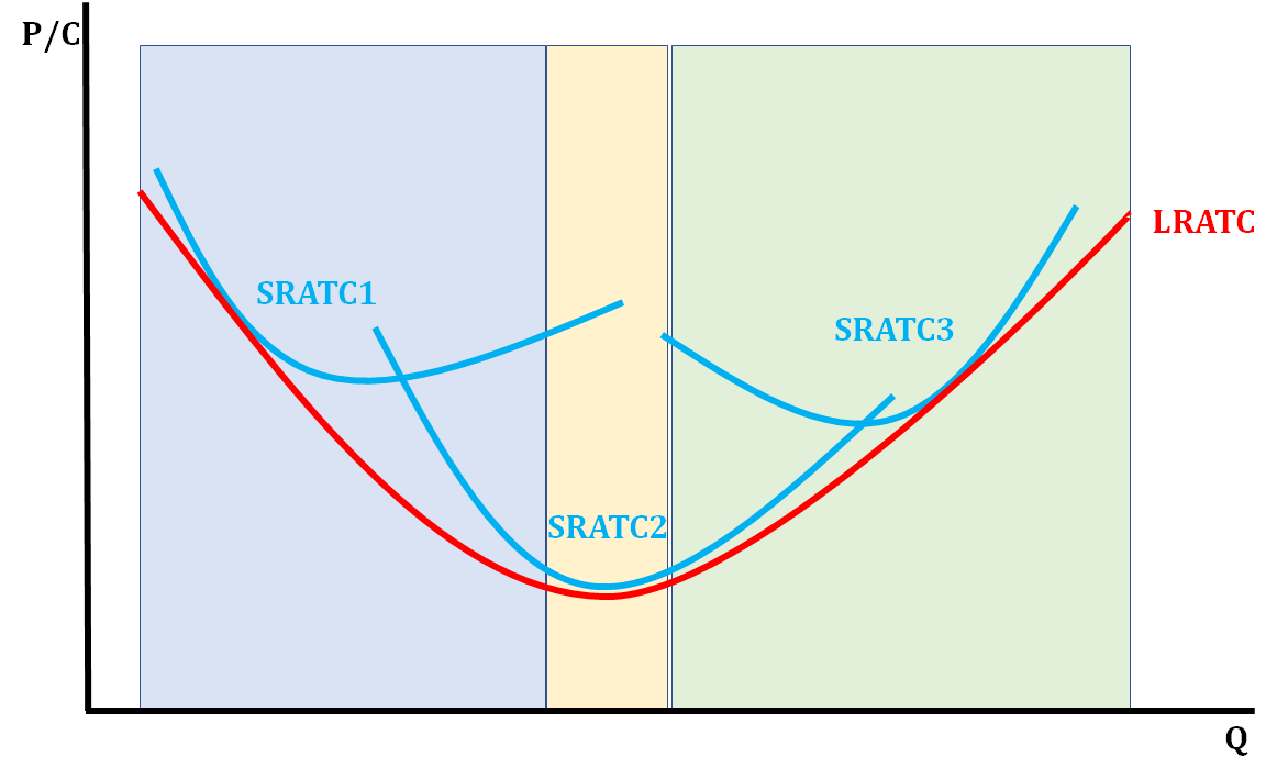
The light blue area represents economies of scale because as output is increasing, costs are decreasing. The light yellow area represents a constant return to scales because as output continues to increase, costs remain constant. The light green area represents diseconomies of scale because as output increases, costs rise.

3.4 - Types of Profit

In economics, there are a variety of different ways to represent profits. These different methods of calculating profits vary based on what type of costs are being considered in each situation. Profit, in general, is the difference between total revenue and total costs (provided total revenue is greater than total costs).

• Accounting profit represents a firm's total revenue minus the firm's explicit costs.

• Economic profit represents a firm's accounting profits minus the firm's explicit and implicit costs. While accounting profit factors in only the explicit costs, economic profit includes implicit costs, and therefore factors in the opportunity costs lost by not pursuing other opportunities.

• Normal profit occurs when a firm's economic profit is zero. So for example, if a firm's total revenue is $100,000 and the total of that firm's explicit and implicit costs is $100,000, then the firm's economic profit is zero, and it is experiencing normal profit. When a firm is experiencing normal profit, its accounting profit is still positive. Normal profit is also referred to as "breaking even."

If revenue is less than costs, a firm may experience economic losses. For example, if the total revenue is $80 and the total cost is $97, we have an economic loss of $17.

When a firm is experiencing an economic profit, they can increase their production. If a firm is earning an economic loss, they will most likely respond by decreasing their output.

3.5 - Profit Maximization

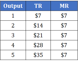
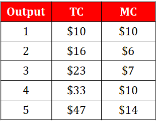
At the point where $\textrm{MR}$ equals $\textrm{MC}$, the costs of producing the last unit of output equals the revenue gained when selling it. At this point, a firm's profit is maximized.

For a firm in perfect competition, $\textrm{MR} = \textrm P$.

Revenue and Costs for an Example Firm

Using this example firm's revenue and costs, we can see that the profit-maximizing quantity is 3 units, where both the marginal revenue and marginal cost equal $7.

MC and the Firm's Supply Decision

If the price of a good increases from $P_1$ to $P_2$, then the profit maximizing quantity rises to $Q_2$. The $\textrm{MC}$ curve determines the firm's $Q$ at any price. (Provided the firm is in perfect competition, as the market sets the price).

3.6 - Firms' Short-Run Decisions to Produce and Long-Run Decisions to Enter or Exit a Market

Shut-Down Rule

A shutdown is a short-run decision not to produce anything because of market conditions. The shutdown rule states that a firm should continue to produce and operate so long as price is equal to or above the firm's AVC.

• Cost of shutting down: revenue loss = $\textrm{TR}$

• Benefit of shutting down: cost savings = $\textrm{VC}$
  • Firm still has to pay $\textrm{FC}$ (rent, electric, other fixed expenses)

• If $\textrm{TR} < \textrm{VC}$, the cost of shutting down is less than the benefit, and a business should shut down.

• Dividing both sides by $Q$ nets the "decision rule"

  $$\frac{\textrm{TR}}Q \lt \frac{\textrm{VC}}{Q}$$

  $$⁍$$

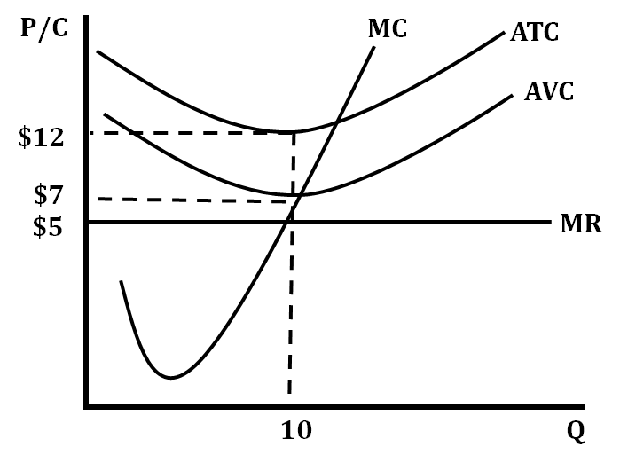
Because on the graph above, the profit maximizing quantity (where $\textrm{MR} = \textrm{MC}$) is below the $\textrm{AVC}$ curve, the firm should choose to shutdown and not produce. If the profit maximizing quantity is anywhere above the $\textrm{AVC}$ curve, the firm should produce.

The Irrelevance of Sunk Costs

A sunk cost is a cost that has already been committed and cannot be recovered.

Sunk costs are irrelevant to the shutdown decision, as you have to pay them regardless of your choice. $\textrm{FC}$ is a sunk cost, as the firm must pay these costs regardless of if they choose to shut down or not. Therefore, $\textrm{FC}$ should not be factored in to the decision to shutdown.

Long-Run Decisions to Enter or Exit the Market

Long-Run Decision to Exit

• Cost of exiting the market: revenue loss = $\textrm{TR}$

• Benefit of exiting the market: cost savings = $\textrm{TC}$
  • There are no $\textrm{FC}$ in the long run

• Therefore, a firm will exit the market if $\textrm{TR} \lt \textrm{TC}$

• Divide both sides by $Q$ to write the firm's decision rule:

  $$\textrm{Exit if:} \quad P < ATC$$

Long-Run Decision to Enter

• In the long run, a new firm will enter the market if it is profitable to do so: if $\textrm{TR} > \textrm{TC}$.

• Divide both sides by $Q$ to express the firm's entry decision as:

  $$\textrm{Enter if:} \quad P > ATC$$

3.7 - Perfect Competition

Characteristics of Perfect Competition

• Many, small firms in the industry

• Firms are "Price Takers"

• Low barriers to entry

• Firms break even in the long-run

• Products sold are identical

• No non-price competition

• Firms are perfectly efficient in the long-run

Assumptions in Market Supply

1. All exisiting firms and potential entrands have identical costs.

2. Each firm's costs do not change as other firms enter or exit the market.

3. The number of firms in the market is:
   1. Fixed in the short run
   2. Variable in the long run

Side-by-Side Graphs of Perfect Competiton

Since firms are price-takers in perfect completion, a firm's MC and MR graph is directly related to the market supply and demand graph. The part of the MC curve that is above the MR curve is the same as the firm's supply curve.

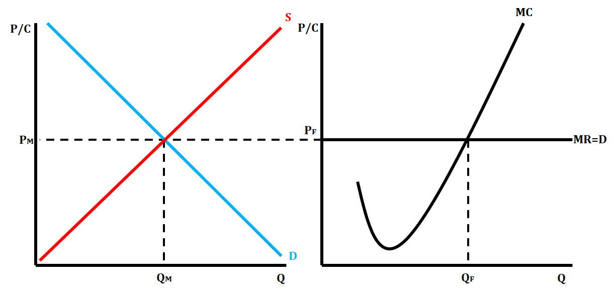
In a perfectly competitive market in the short-run, a graph can display three possible scenarios. They can show a short-run profit, short-run loss, or short-run shutdown.

Short-Run Profit

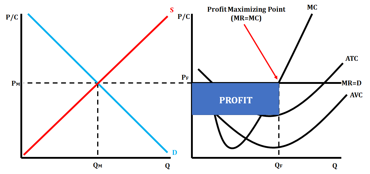
When a firm is making a short-run profit, its profit per unit = $\textrm P - \textrm{ATC}$. Therefore, the firm's total profit is equal to $(\textrm P - \textrm{ATC}) \times Q$.

Short-Run Loss

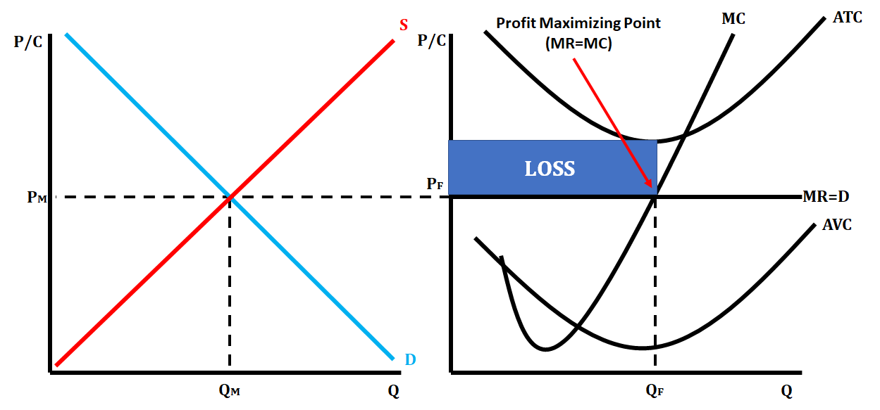
A short-run loss is shown when the ATC is located above the price line at the profit-maximizing point, and the AVC curve is located below the price line at the profit-maximizing point.

When a firm is making short-run losses, its loss per unit equals $\textrm{ATC} - \textrm P$. Therefore, the firm's total loss is equal to $(\textrm{ATC} - \textrm P) \times Q$.

Short-Run Shutdown

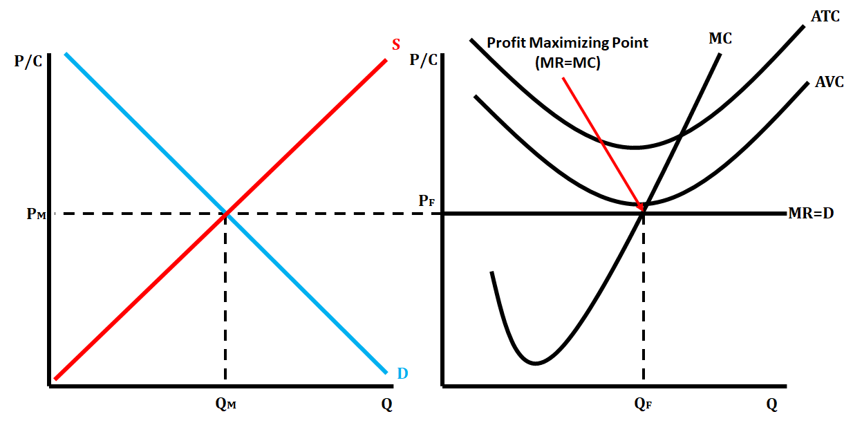
A business will shutdown when both ATC and AVC are located above the price line at the profit-maximizing point, as shown above.

Long-Run Perfectly Competitive Graph

When a perfectly competitive market is in long-run equilibrium, we show this on the side by side graphs by having ATC tangent to the price line at the profit-maximizing quantity (MR = MC). When a perfectly competitive market is in long-run equilibrium, it is both allocatively efficient and productively efficient. On a graph, allocative efficiency is P(MR) = MC, and productive efficiency is P = minimum ATC.

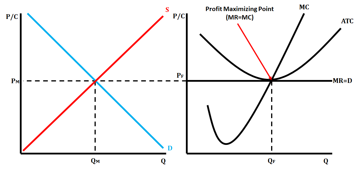
Shift from Short-Run to Long-Run Equilibrium in a Perfectly Competitive Market

When a short-run perfectly competitive market is earning either a profit or loss, firms will want to either enter or exit the market, thus market shifting the market from short-run to long-run.

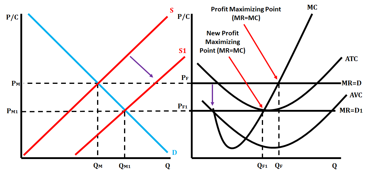
When a firm is earning a profit, this provides an incentive for firms not already in the industry to enter because of the possible profit. This will cause the supply curve to shift right due to the increase in supply, which will lower the market price and in turn lower the price for each firm.

This can be illustrated on a graph by shifting the price line down to become tangent with ATC. The profit-maximizing quantity for the firm will decrease. The market quantity will increase as there are now more firms in the industry, but each individual firm is supplying less of that overall quantity.

The below graphs show how a perfectly competitive market goes from a short-run profit to long-run equilibrium.

Since firms joining the market reduces the profit made by each firm, eventually some firms will be incentivized to leave the market, repeating in a cycle until the remaining firms earn zero profit:

The Zero-Profit Condition

• Long-run equilibrium: The process of entry or exit is complete, and remaining firms earn zero economic profit.

• Zero economic profit occurs when $\textrm P = \textrm{ATC}$.

• Since firms produce when $\textrm P = \textrm{MR} = \textrm{MC}$, the zero-profit condition is where $\textrm P = \textrm{MC} = \textrm{ATC}$.

• Recall that MC intersects ATC at the minimum ATC.

• Hence, in the long run, $\textrm P = \textrm{minimum ATC}$.

Shift from Long-Run to Short-Run back to Long-Run

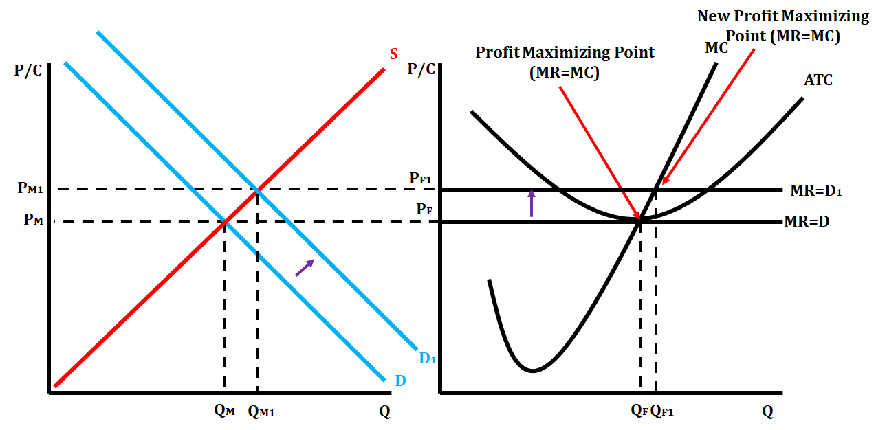
A market may be in long-run equilibrium, and then experience a change in demand in the market. This shift of demand moves the market into short-run, and then it has to readjust back to long-run.

Let's show how this occurs when there is a scenario that increases demand. We'll use the market for apples.

Step 1

A market is in long-run equilibrium, when a change in market demand causes the price of the good to increase. We show this on the firm graph by shifting the price line up and identifying the new profit-maximizing point for the firm ($\textrm{MR} = \textrm{MC}$). This causes the firm to go from long-run equilibrium to short-run profit since the price line is above the ATC curve.

Step 2

Now that the perfectly competitive market is earning a short-run profit, individual firms are incentivized to enter the market. This makes the supply curve shift right, causing the equilibrium price to decrease. This will cause the price line to drop on the firm graph and cause the profit-maximizing quantity to return to the original one in the firm.

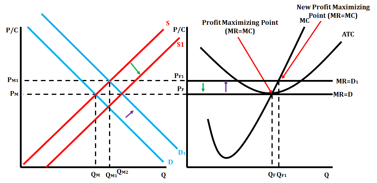
This can happen anytime a perfectly competitive market starts in long-run equilibrium and gets moved to short-run. The market always has to readjust to long-run equilibrium.

Changes Due to the Assumptions of the Perfect Competition Model

1. Firms have different costs
   • A $P$ rises, firms with lower costs enter the market before those with higher costs.
   • Further increases in $P$ make it worthwhile for higher-cost firms to enter the market, which increases market quantity supplied.
   • Hence, the $\textrm{LR}$ market supply curve slopes upward.
   • At any $P$,
     • For the marginal firm, $P = \textrm{minimum ATC}$ and $\textrm{profit} = 0$.
     • For lower-cost firms, $\textrm{profit} > 0$.

2. Costs Rise as Firms Enter the Market
   • In some industries, the supply of a key input is limited.
   • The entry of new firms increases demand for this input, causing its price to rise.
   • This increases all firms' costs.
   • Hence, an increase in $P$ is required to increase the market quantity supplied, so the supply curve is upward-sloping.

Conclusion: The Efficiency of a Competitive Market

• Profit Maximization: $\textrm{MR} = \textrm{MC}$

• Perfect Competition: $P = \textrm{MR}$

• So, in the competitive equilibrium, $P = \textrm{MC}$

• Recall, $\textrm{MC}$ is cost of producing the marginal unit. $P$ is the value to buyers of the marginal unit.

• For a firm in a perfectly competitive market, price = marginal revenue = average revenue.

• IF $P > \textrm{AVC}$, a firm maximizes profit by producing the quantity where $\textrm{MR} = \textrm{MC}$